Why Data Matters
Data drives decisions, gives insights into how time or money is spent, tracks budget status, and shows trends throughout history. There are also many ways that data can be shared or displayed – in tables, showing comparisons, converting to a multitude of different graphs, illustrated in eye-catching graphics. The possibilities are endless.
The key to data is to know how to use the tools available for organizing and sharing it – like Excel and Google Sheets. This article will be focused on how to do things in Excel, but the actions can be translated for use in Google Sheets if that is the program you have available.
Excel Terminology
Workbook or Spreadsheet
The entire Excel file is called a workbook and will have a .xlsx or .xls file suffix.
Sheet or Tab
Within a workbook, you can have multiple sheets or tabs of data, shown across the bottom. These can be similar sets of data, different variations of the same data, or completely different data – it’s up to you!
To add a sheet to a workbook, click the + right next to “Sheet 1” at the bottom. You can also change the name by double-clicking or right clicking and selecting “Rename.” I’d suggest keeping the number of tabs below 20, as even a 20-sheet file can contain A LOT of data to manage!
Columns
Columns go left to right, labeled with a letter across the top (A, B, C, D, etc).
Rows
Rows go top to bottom, labeled with numbers (1, 2, 3, 4, 5, etc)
Cell
A cell is a specific box of data known as the corresponding column and row (ex: A13)
Formula
Within each cell, you can add a formula that will do specific actions to a group of cells you select. One of the most common formulas is the sum formula, used to add up the total of a series of cells.
Making data “pretty”
A few simple tweaks of how the data is presented can make a significant difference in how people take it in. It can be as simple as consistent formatting or presenting the data in a more digestible format.
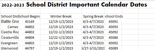
After making everything the same font (Calibri), merging the title cells to go across the whole data set, bolding the header/top columns, ensuring all the dates entered are formatted as dates, and adjusting the column widths so the first column (School District) is all readable, the dates columns are all the same size, and adding borders to the cells, the same data looks cleaner and much more readable.
Before and After
Drag your mouse to see the differences after formatting has been applied. Doesn’t it look so pretty and clean this way?

So how can you make these simple adjustments?
Just by making some simple, visual adjustments, your data will be much easier to read and digest.
Fonts
One of the easiest ways to make data pretty is to use one font family. If you have brand fonts for your district/agency, use these or a simple sans serif font that is accepted by Microsoft and Google products like Calibri or Arial so it can be easily viewed by anyone opening your file.
In the above example, Calibri was the font used, with all text in the table at 11 pt, the title at 18 pt, and both the title and column headers were bolded.
To change the font and text size of your data, select all desired cells (or the whole sheet by selecting the triangle in the top left corner) then change the font to your desired font.

Bolding certain columns or rows is a great way to distinguish these cells as category headers or to call out specific data to pay attention to.
Increasing the size of the text is a great way to distinguish titles.
Color
You can also add some subtle colors to your tables (notice, I said SUBTLE – don’t go overboard ???? by adding a background color to select cells. I tend to either do the column headers or row headers, and muted colors so the text inside each cell is still easily readable.
Adjusting Column Widths and Row Heights
There’s a few ways to do this, depending on how you want the columns or rows set.
This can be helpful for not only aligning data, but also to make it fit on one page if it’s just slightly larger (sizing down) or adding white space to view the data (sizing up) more easily.
In this example, the School District column has a width of 25 and the 4 date columns are a width of 15 each. The row heights were adjusted automatically based on the font size of each row.

If you double click on the column letter at the top of a corresponding column of data, this will make sure all data in a column of cells is visible (based on the longest cell). If you have a lot of data/words in one cell, this could make the entire column extremely long, so it’s not always the best choice.
For rows, adjusting the font size of a cell or row of cells will adjust the row height automatically to accommodate.
If you want to set columns to a certain width of your choosing, select the corresponding column letter and right click. Select “Column Width” and adjust in the pop-up window. For multiple columns, select all column letters you want across the top, right click, select “Column Width” and enter your desired value.
For rows, it’s similar but after right clicking, select “Row Height” and adjust.
Formatting Data in Cells
Cells can be formatted in many ways: as numbers (with or without decimals), dates, percentages, accounting and currency are some of the most common.
In this example, all dates were selected as “Date” and then M/D/YYYY was the specific date display option selected (show in example as 3/14/2012).
To format a cell or group of cells, select the cells you want and right click. Select “Format Cells” and then select your desired formatting from the pop-up window.

Merging Cells
This allows you to spread the data in one cell across multiple cells (can be adjoining cells in columns, rows, or both). It’s handy for adding a title to the data set/table, extending a header across multiple columns, or combining rows.
To merge cells – select the cells you want to merge (highlighted in yellow below), then select the “Merge & Center” button in the tools ribbon. It will automatically center the information across the newly merged cells.

Keep in mind if info is in multiple cells, only the info/data in the top left cell will be kept.
Adding Borders to Cells
While you see the cells outlined in light gray when looking at them in the actual excel file, the outlines (also called borders) are not automatically added when a sheet is printed. Adding borders to the cells is a simple way to make your table look finished and it makes it easier for anyone to read along and follow the data across rows or down columns.
In this example, “All Borders” were added to the data set (does not include the merged title cells)
To add borders to cells, select the desired cells (usually everything in a data set), then the little cell box under your font. Select the type of border desired.
All Borders is the most common; Outside Borders or Thick Outside Borders will add a border around only the outermost perimeter of all cells selected.
If you’d like to have more formatting options, select “More Borders” at the bottom – here you can change the color of the border, thickness, type of line, etc.

What if I have a lot of number data (like money), how can I make that pretty for the people who dislike Excel with a fire-y passion? And what tricks can help me?
I’m glad you asked! Numbers/money and spreadsheets go hand in hand and a few simple tips and formulas can change your life when given a pile of data to share.
If you deal with numbers or money (such as tracking budgets or revenue), the sum formula will be your best friend! It does calculations for you, and in a split second – its seriously life changing!
How do you use this magic formula? Well, first you need some data, here’s an example >

The Sum Formula
The Totals listed across the bottom are all created using the sum formula. For easy reference, I will be indicating what to type with bold and italics. You do not need to do the same when typing into Excel.
In the cell you want to show a total or sum, type =SUM( then select the group of cells you want to add together, and hit enter – it will automatically close your parentheses, or you can do it yourself by typing ) after the cells before hitting enter. Do not add spaces in between, as this will break the formula.

In this case, I want to add cells B5 to B16 together to show me the External revenue for our 2021-2022 fiscal year (September-August), which shows as B5:B16.
If you click on cell B18 (where we entered the sum formula) it now shows =SUM(B5:B16) and you see the cells being added together are boxed in blue box and cell B18 has a green box around it.
More Tricks
Want to know a totally awesome trick? If you click on the bottom right corner of the green box (the cell you typed the sum formula into) and drag it across the row, it will use that same formula for the next column(s) of data. It will look like this, and will populate the cells with their corresponding totals:

I didn’t retype the sum formula into cells C18, D18 or E18 – I just dragged the formula from B18 over, and it adjusted to sum the data in the same column! Magic!
It is always good to double check that the data being added together is correct – click on the total cell to see what data is included.
You can even add items together that aren’t all in connecting columns or are even from different sheets. After typing in the formula =SUM( select the cells you want to sum.
If selecting different groups of cells on the same sheet (in this example B5:B16,C5:C16,G5:G16,H5:H16), hold the Control key when selecting each of the cells, this will add each grouping of cells in a new color box, and separate them with a comma in the formula. You’ll notice each grouping of cells is color-coded to their corresponding box around the cells.

If selecting cells from another sheet, type in the formula, then click over to the sheet you want, and select the cells to add together. In this case, the formula shows it’s adding from Sheet4, if I had changed the name it would say that name.

What about if I want to subtract, multiply, or divide numbers in cells? Or show numbers as percentages?
This is where = and ( ) are your friends!
Subtraction
To subtract, type = select the first cell, type – and select the second cell, then press enter.
In this case, I wanted the yearly total (D16) minus August’s total (D14). When I press enter it gives me $414,636.05. The green boxed cell shows the formula of =D16-D14.

To subtract a group of numbers, simply add ( ) around the grouping of numbers and make sure to add the function you want within the ( ). Think about the Order of Operations from math (PEMDAS) where anything inside parentheses gets calculated first). In this case, I wanted to subtract June, July, and Aug from the total. The green boxed cell shows =D16-(SUM(D12:D14)) – make sure you close the parentheses.

Multiplication
To multiply, type = and either the cell or a number, then * and either a cell or a number, then enter.
In this case, I wanted to multiply a cell (E16) by 125, so the green boxed cell shows =E16*125, and the total is 96406.25.
If the 125 is a dollar rate, and I want to show the total in dollars, I would select the cell (E19) and change the formatting to be either Accounting or Currency, with 2 decimal places and the US dollar symbol $.
NOTES: Accounting just shows the number as a dollar value. Currency shows negative values in red or ( ), depending on which you choose.

Division
To divide, type = and either a cell or a number, then / and either a cell or a number, then enter.
In this case, I wanted to divide September’s total (D3) from the full year total (D16, or 462730.79), so the green box shows =D3/462730.79. I could also have selected the total cell (D16) – either way works.

I wanted to see the values in the F column as percentages, so after adding the formula into each cell in the column, I selected those cells and formatted to Percentages with 2 decimal places.

A benefit of typing in a number vs selecting a cell in some cases is you don’t have to adjust the formula once you’ve dragged it into other cells.
If you used the specific cell for the total (D16), you would need to adjust each following cell to still divide by D16 – it’s noticeable if the formula is incorrect (like dividing by a cell that doesn’t have a number in it) because you’ll get the error. In this case, the cells show #DIV/0! because you can’t divide it by 0 or nothing.
Cell F6 shows a number because it’s dividing D6 by D19, which does have a value, just not the correct value we wanted that is in D16

Conclusion
These are just a few of the ways I use Excel daily. And I know there’s so many more ways to utilize Excel to make your job easier, what I showed here is just a tiny scratch on the surface!
Also, keep in mind sometimes a certain set of features just doesn’t mesh as well with other programs. For example: I don’t use the graphs features in Excel very often, because our Design team is great at adding graphs or other graphics to design layouts, and it’s easier for them to create it within the design software from the data I provide, rather than copying a graph over and then having to reconfigure everything because the formatting didn’t translate.
If you get stuck, there’s always help. I’ve found the easiest way for me to learn how to do something new in Excel or if I want to know how to do something specific is to ask someone I know, ask Google as there’s many great tutorials (in written and video form), attend a training, or use a platform like LinkedInLearning with classes that build upon each other and your understanding of programs.
Like I said earlier, data isn’t scary if you know what to do with it!